Analysis of Variance

(Chapter 10 in Zar, 2010)

We now have a tool (the 2-sample t-test) that will allow us to compare two sample means. More often than not, however, we design experiments that require the comparison of more than two groups. While it might seem logical that we could use the t-test multiple times to accomplish such a comparison (e.g., compare among A, B, and C by comparing A to B, A to C, and B to C), this creates a serious issue with the type I error rate, α. Every time you conduct a comparison, you have a 1 in 20 chance of committing a type I error. Multiple analyses on a single data set compounds that error rate. In the example mentioned previously, the 3 comparisons would result in a type I error rate for the overall comparison of 0.15.

No problem...we'll just divide α by 3 to find our critical value, right? Actually, that creates a different problem. Decreasing α for each individual test increases the type II error rate for each of the individual comparisons. While there are corrections that operate on the principle of dividing the type I error rate, such as the Bonferroni correction, it is far better to utilize a single analysis to compare 2 or more means that is covered by a single type I error rate, such as the venerated analysis of variance (ANOVA).

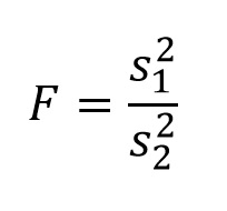
The probability distribution that ANOVA relies upon is called the F-distribution (after Sir Ronald Fisher). The F-distribution is a distribution of variance ratios drawn from a single statistical population. In other words, each observation in the distribution is the result of drawing 2 samples from a single statistical population, calculating the variance (s²) of each sample, and dividing one by the other:

For the example below, the 5000 observations (the ratio of 2 sample variances is one observation, so 10,000 samples were drawn in total) were drawn from from a normally distributed population with μ = 10 and σ = 2 (the R program can be viewed HERE):

If the animation does not work, or if you want to examine the individual graphs, they can be viewed HERE.

Question 1: Why is the F-distribution centered around a value of 1?

You can see that the sample sizes used for the samples from which the variances (and thus the resulting variance ratios) were calculated influence the shape of the distribution. In this example, the same sample size was used for both the numerator and denominator variances, but (fortunately, as you will see) this is not a requirement. Unlike the previous theoretical ditributions that we have employed (the t-distribution and the χ²-distribution), the shape of the F-distribution is influenced by both numerator and denominator degrees of freedom. In this example, these correspond to n₁ - 1 for the numerator degrees of freedom and n₂ - 1 for the denominator degrees of freedom.

Examine Table B.4 in your textbook (starting on p. 680 in the 5th Edition), which contains the critical values for the F-distribution. The first column of the table contains the denominator degrees of freedom (v₂), and there is a separate table for each value of the numerator degrees of freedom (v₁). It probably has occurred to you that this might have some utility in testing assumptions of homogeneity of variance, which is true, but unfortunately the assumptions required to apply the F-distribution to that question make that approach of limited utility, and so we will stick with Bartlett's test when it is important, and Hartley's F_max test for the examples you will analyze in this class. No, I am not implying that this class isn't important...

If you have been nodding and smiling up until this point, you have overlooked a very important paradox. The goal of ANOVA is the comparison of sample means, but it relies on the distribution of a variance ratio. Knowing that our most recently applied test for comparing means, the 2-sample t-test, requires the assumption of homogeneity of variance should indicate to us that it is quite possible for statistical populations with different means to have the same variance. So how is it possible to compare means with a variance ratio?

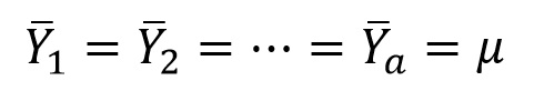
Examining the problem a different way, how do we test the null hypothesis:

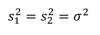
Using a distribution that is the null expectation for:

???

via GIPHY

The solution to the paradox involves breaking down the value of an observation into its various determinants. Every observation, Y belongs to a statistical population with a mean of μ, even though we likely have no idea what that population mean might be. That observation deviates from that mean as the result of individual variation, which we will denote as ε. ε is essentially a deviate (observation minus the population mean). If we apply some fixed treatment to an experimental unit, that treatment should add additional variation, which we will denote as α. For example, if you are shorter than the average height for the statistical population to which you belong, one basis for this could be genetic, and so (all else being equal) your height would be expected to deviate from the average by ε. However, this deviation could be altered by having smoked a lot of cigarettes and drank a lot of coffee in kindergarten. That alteration would be expressed as α.

Note that this is a different use for the same symbol that we used to denote type I error rate. They are not directly related. Later on, for regression analysis, we will use the same symbol to denote the Y-intercept. This means that you are going to have to pay careful attention to context!

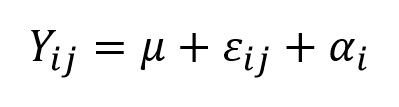
Where Y_ij is the jth observation in group i, and deviates from μ (the mean of the population from which all individuals in all groups were drawn) by the individual variance component ε_ij. The variation added by the treatment to which the group was exposed is denoted as α_i.

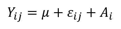
Variation added by random effects (treatment effects are considered fixed effects) is treated the same way, except that it is denoted as A_i:

It is the variance components ε and α that are used to create a variance ratio that will be compared to the null expectation of the F-distribution as:

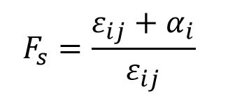
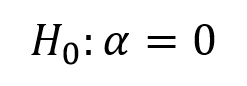
The individual variation is included in both the numerator and denominator, but the treatment variation (or random effect variation) is included only in the numerator. If there is no variation added due to treatment effects, i.e., if α = 0, then the numerator and denominator estimate the same thing, and the ratio should fit the null expectation. So, even though the null hypothesis we report for ANOVA is:

The null hypothesis that we really are testing is:

The good news is that this makes ANOVA a one-tailed test, regardless of the circumstances. The bad news is that you now have to explain why...

Question 2: Explain why the application of the variance ratio, F_s, as described above, is always a one-tailed test.

ANOVA with a fixed independent variable (H₀: α = 0) is referred to as model I ANOVA, and ANOVA with a random independent variable (H₀: A = 0) is referred to as model II ANOVA. There is no difference between the 2 in terms of how F_s is calculated, only in how we structure the null hypothesis. The distinction between model I and model II ANOVA will, however, take on special significance next week when we address n-factor ANOVA, where there is more than 1 independent variable.

Speaking of F_s, how do we go about calculating it such that the numerator estimates ε + α, and the denominator only estimates ε? Let's start with the denominator. The differences between the means of distributions of treatment groups should be the result of α, but individual variation (ε) should not vary among the groups if the experimental design has no bias. In other words, treatment effects should shift the central tendency, but not the dispersion around that central tendency. Thus, we should get a good estimate of ε by examining the variation within each group, and a better estimate by averaging across the groups. We can refer to this as within group variation because the components of the estimates come from within the groups.

Often, however, our sample sizes are unequal, and so we need a weighted average variance, because larger sample sizes produce better estimates. To do this, we could multiply each variance estimate by the sample size used to generate it, and divide the result by the sum of the sample sizes.

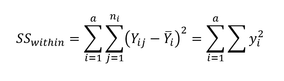
We are going to take a different approach that accomplishes the same thing. The reason for this is that it will allow us to construct an ANOVA table step by step, which is how software packages display the results of ANOVA. We will approach the calculation of average within-group variance by first calculating the within-group sum of squares, also referred to as error sum of squares in your textbook. Within-group sum of squares is simply the sum of ∑y² across all groups (the sum of the sums of squares...):

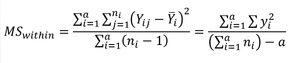
The denominator of F_s is referred to as within-group mean squares (MS_within) or error mean squares (we shall use the former), and is calculated by dividing SS_within by the appropriate degrees of freedom (the sum of the degrees of freedom for each group):

Again, the calculation is simple: the equation on the left indicates subtracting 1 from each of the sample sizes and summing them together, and the one on the right indicates that the sample sizes are summed, and the number of groups being compared be subtracted from that sum. MS_within then, is simply:

Or, if you prefer the busier versions:

This gives us the denominator for F_s, which you may recall is our estimate of ε. For the numerator, which estimates ε + α (where α is variance added due to treatment in a model I ANOVA, not type I error rate), or ε + A for model II ANOVA, we need an independent estimate of variance that includes variance added due to treatment. We already have used the individual observations for MS_within, and so employing them again would not give us an independent estimate. Using the sample means, however, would give us an independent measure, and one that included treatment effects (ε) or random effects (A) if these effects contributed to the differences among the means. The first step is to calculate a grand mean, which we will denote as a Y with 2 bars over it (the use of a subscript in your textbook to distinguish sample means from grand means seems likely to lead to confusion):

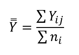
As the name implies, this is the overall mean, determined by summing all of the observations across all of the groups, and dividing by the total number of observations. It may occur to you that you also could take the average of the sample means, which is true, but only when the sample sizes are all equal. The =AVERAGE() function in Excel works just fine when you highlight rows of observations across more than one column (i.e., a matrix), so calculating the grand mean by highlighting all of the observations is a simple approach.

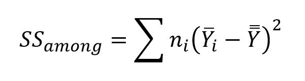
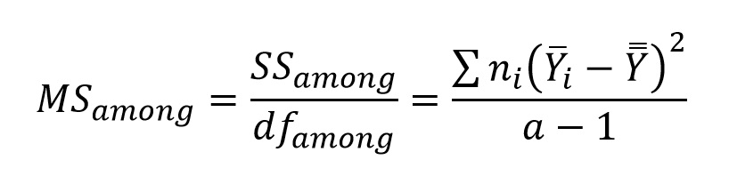
To get our estimate of variance using the means, we calculate the among-group sum of squares (SS_among) as the squared deviations of sample means from the grand mean (essentially treating the sample means as observations), multiplying each deviation by the sample size used to generate the sample mean:

Because there are a sample means (remember that a is the number of groups in the comparison), the degrees of freedom (df_among ) for the among-group mean squares (MS_among) are a - 1, and so the numerator of F_s is calculated as:

Thus, our variance ratio F_s is calculated as:

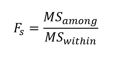
And the resultant value compared to F_crit at α(1) = 0.05, at df_among numerator degrees of freedom (v₁ in Table B.4) and df_within denominator degrees of freedom (v₂ in Table B.4). Remember that because the other α, variation added due to treatment, or A (variation added due to random effects) always is added to the numerator only, ANOVA is always a one-tailed test. It is important to note that rejecting the null hypothesis will not tell us which means differ from each other; it will only tell us that there is a difference in at least one of the means. Finding which means differ from each other involves analyses referred to as multiple comparisons, which we will get to shortly.

As mentioned previously, the calculations are the same for both model I (fixed effects) and model II (random effects) ANOVA, and so we can apply the above calculations to our examples without worrying about distinguishing between the two for the time being.

In order that you may become familiar with the presentation of an ANOVA table, you will be presenting your results in this format for the remaining questions. The following table serves the dual purpose of showing you the format for the table, and providing you with a quick-guide to the necessary calculations:

Of course, you will be filling in the values, for df, SS, MS, and F_s, and not recopying the formulas...

Download this week's Excel workbook HERE.

The first worksheet ("Example10.2"), not surprisingly, contains the data from Example 10.2 (page 201 in the 5th edition). Work it through to make certain that you understand the calculations. Do not use the formulas that they use in the example! Use the formulas that have been provided above. The methods in the text are shortcuts that hide the actual basis for the calculations. You should, however, arrive at the same result, which will tell you whether you have applied our formulas correctly or not, which is the whole point of starting with an example from the text.

The data in the second worksheet ("squirrel") come from an experiment testing whether northern flying squirrels hunt by scent. The time spent digging was recorded for individual squirrels in pens with a buried marble, a buried marble covered by a log, a buried truffle, and a buried truffle covered by a log.

The third worksheet contains data from a gut content analysis of alpine newts, comparing the number of Daphnia longispina found in each digestive tract for sample of newts collected in June, August, and October of the same year.

Question 5: Present the ANOVA table for the newt data. Is there a significant difference in the mean number of D. longispina among the months?

Not surprisingly, ANOVA is a parametric test, which means that we need to address the assumptions of ANOVA...

Send comments, suggestions, and corrections to: Derek Zelmer