Assumptions of Analysis of Variance

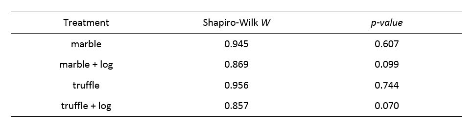
Analysis of variance shares the assumptions of normality and homoscedasticity (homogeneity of variance) with the 2-sample t-test. The assumption of normality must be tested within each group, requiring that the Shaprio-Wilk test be conducted a times. As promised, I have conducted the Shapiro-Wilk tests for the analyses that you have conducted thus far. For the squirrel data, the results are:

And for the newt data, the results are:

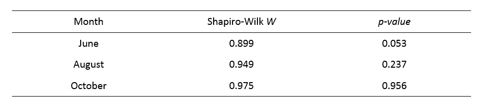
Question 6: Do all of the samples for these 2 analyses meet the assumption of normality?

The homogeneity of variance assumption can be tested using our old friend, Hartley's F_max -test. To refresh your memory, the test-statistic F_max is calculated by dividing the highest sample variance from your groups by the lowest sample variance from your groups, and comparing that ratio to the appropriate value from THIS table. Remember to base your degrees of freedom on the smallest sample size from the two groups that you use to generate the ratio, not from the overall smallest sample size.

Question 7: Do the data from any of the analyses you have conducted thus far violate the assumption of homogeneity of variance?

Hopefully it has occurred to you that the usual procedure would be to first test the assumptions of a given analysis before applying that analysis. Let's adopt this common-sense approach to the 5th set ("sculpin") of data (don't panic, we will come back to the 4th set). In this experiment, the question under investigation was the importance of visual and chemical cues on predator avoidance by the slimy sculpin. Cages containing nothing (no cues), a small trout (chemical cue, but not a large visual cue) or a large trout were distributed randomly among likely sculpin habitats, and the habitats sampled for sculpin (by electroshocking) after a few hours of exposure to the cages. The Shapiro-Wilk results are as follows:

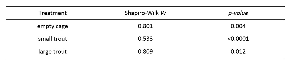
These values suggest that our data are pretty far away from meeting the assumption of normality. This gives us the opportunity to apply a nonparametric equivalent of ANOVA: the Kruskal-Wallis test. This analysis is covered in section 10.4 of the 5th edition of your textbook. Take a moment to read through the procedure. Not too cumbersome, but still somewhat inconvenient. The 4th worksheet ("Example10.11") in this week's Excel workbook contains the ranks from Example 10.11 (imagine that). Instead of applying the Kruskal-Wallis test as outlined in your textbook, do an ANOVA on the ranked data, following the same procedure that you used for the first 3 analyses. Use Table B.4 to determine the boundaries for your p-value.

Question 8: Based on Table B.4, between what range of probabilities does the p-value from the ANOVA on ranks fall? How does this compare with the range given in Example 10.11 for the Kruskal-Wallis test (the F-value using Equation 10.43) on the same data?

One of the best-kept secrets in biostatistics is that conducting an ANOVA on ranked data is the equivalent of the Kruskal-Wallis test (Iman et al., 1975). With that in mind, perform a nonparametric ANOVA on the sculpin data by conducting a conventional ANOVA on the ranked data.

Question 9: Present the ANOVA table for the ranked sculpin data (you will have to generate the ranks yourself). Is there a significant difference among treatments?

I can think of very few instances (except when only 2 samples are being compared) where one would not be interested in determining which means differed. The appropriate analyses for this are referred to as multiple comparisons...

Send comments, suggestions, and corrections to: Derek Zelmer