Open up Excel, which should bring you to a blank spreadsheet. Note that the columns are delineated with letters, and the rows are delineated with numbers. You can move among the cells using the arrow keys, the "page up" and "page down" keys, and/or by clicking on a cell with your mouse.

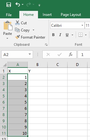
In cell A1 type "X" (do not type in the quotes) and in cell B1 type "Y". To get the cell to accept your entry, either hit "Enter", which will move you one cell down, or use one of the arrow keys to move away from the cell. Throughout the semester, we will be using the letter "X" to denote the independent (or manipulated) variable, and we will be using the letter "Y" to denote the dependent (or responding) variables for our observations.

Our first step will be to fill the first column (A2 to A11) with the numbers 1 through 10. We could simply type these numbers into the cells, but there is an easier way to do this, especially for large series of numbers. First, type the number "1" into cell A2, and hit "Enter". Then, highlight 10 cells beneath the "X" label, including cell A2, which tells the fill function what our starting number is. If you are not fond of counting, you can highlight more than 10, because you can supply the fill function with a stopping number.

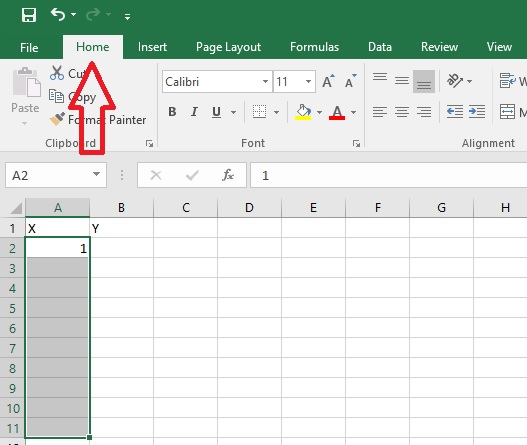
In the bar across the top of the sheet, click on the "Home" tab:

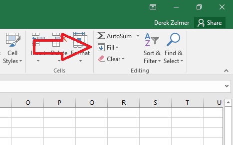
Look to the far right on the tool bar that appears and click on "Fill":

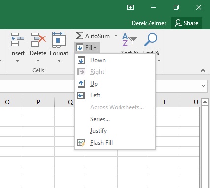
This should bring up the following menu:

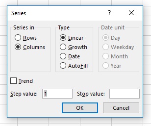
The selection should be set for "Columns" and "Linear", which are the settings that we want. "Step value" determines the interval between the values. In this case, the interval is one. If you have highlighted more than 10 cells, then type "10" into the "Stop value". Click "OK", and the cells in column A should fill with the correct values:

At the bottom left corner of your spreadsheet, click on the "+" sign to open a second sheet:

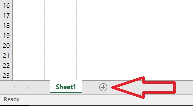
Label the sheet the same way, and fill in a series of numbers for the X variable starting at 5, and ending at 50, by setting the "Step" value to "5".

If you have not been saving regularly, take the time to save your workbook now. If you are working in the computer lab, save your work onto the "J:" drive, or any cloudy thingy to which you have access. After 90 minutes of inactivity, the computers in the computer lab will shut down, and delete anything that you have saved. Click the "File" tab on the left side of the upper tool bar, and on the page that comes up, select "Save As" from the menu on the left:

Select a folder in which to save the file, and name the file "yourlastnameex1. For example, I would save the file as "zelmerex1". Once the file has a name, saving it as you work is as simple as clicking on the floppy disc (ask your parents) icon at the top of the workbook:

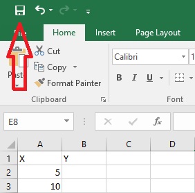
Like voting, remember to save early, and save often.

Now we can work with some simple formulas. In Excel, you can perform mathematical operations on cells, and copy these formulas to repeat the operations. You must always start by entering the "=" sign to let Excel know that you are doing math (even though that is what it was designed for). The symbols for addition and subtraction are "+" and "-" respectively, as you might suspect. The symbol for multiplication is an asterisk ("*"), and you use a forward slash ("/") for division.

=a2^2

Note that you do not have to use upper-case letters to denote columns. As an alternative to typing in the cell coordinates, you also can click on the cell that you want to reference with the cursor after you have typed the "=".

Click on the "Sheet 1" tab at the bottom of the sheet to return to your original spreadsheet.

In cell B2, type the formula shown above to square the value in cell A2, and hit enter. Now click on cell B2 again. Notice that there is a border around the cell, with a dark square in the bottom right corner:

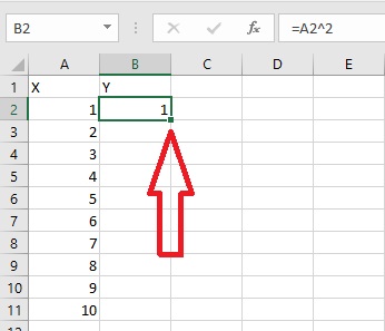
Click on that square, and drag down the column for each cell adjacent to a value in column A, and then let go of the mouse button. You will see that in column B is now filled with values corresponding to the squared values in column A.

Now click on cell B11, and hit "F2" (one of the function keys at the top of your keyboard). It will show you the formula in the cell and place a color coded box to show you the cell referenced by the formula. It also shows you the formula in the formula bar at the top of the page (red arrow):

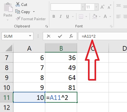
The function key "F2" will allow you to see the reference cells for the formulas, and also allow you to edit your formulas. Note that when copying formulas, it is the frame of reference, i.e., where the referenced cells position is relative to the cell where the formula is, that is important, not the actual row or column designation, or what sheet you are on. To demonstrate this, highlight all the cells in column B that have numerical values, copy them (using Ctrl+C), and then paste them in column C by clicking on cell C2, using Ctrl+V. The values are now the squared values from column B.

There will be circumstances, however, where you don't want the reference point of a formula to change when you copy the formula. In these cases, you can anchor a row, or column, or both, using the dollar sign ($)

We will demonstrate the function of the $ anchor by introducing a new Excel function, which gives you the sum of a row or column of cells. Not surprisingly, the name of the function is "SUM".

Click on the "Sheet 2" tab at the bottom of the page to shift to the second worksheet. In cell A13, type the following:

=sum(a2:a11)

Again, as an alternative to typing the cell coordinates, you can highlight the cells that you want the sum of after you have typed the left parenthesis. Hit "Enter", and you will see the sum of the values in column A. Now, drag that formula over to cell B13, using the same technique that you used to copy the formula that squared the values in column A on sheet 1. That value should be zero because there are no values in the corresponding cells. Use F2 to see the cells referenced in the formula to verify this.

Now we will make use of the anchor symbol, which keeps the reference from changing when formulas are copied. In cell B2, type the following:

=sum(a2:a11)

Notice that you get the same value as you got in A13, because it is the same formula with the same references. Notice also that the value in cell B13 has changed. This is an important feature. Because the value for B13 is determined by a formula, changing a value in one of the reference cells will change the value for B13. This is useful in that correcting an error made at the beginning of a set of calculations will carry that correction through all subsequent calculations, so that you don't have to start over. It can also be dangerous if you make changes as part of a second set of calculations, as the values for the first set will all be changed.

Now drag the formula in B2 down through B11.

Question 1: Why do the values in column B first increase, and then decrease? (Use F2 to help discover what happened)

In cell C2, type the following:

=sum($a2:$a11)

Drag the formula down to C11, then copy column C to column D by highlighting the cells in column C and using Ctrl-C to copy and Ctrl-V to paste, or by highlighting the cells, and dragging to the next column.

Question 2: Why are the values in column D the same as in column C? What did placing the dollar sign in front of the column letter tell Excel to do? (Again, using F2 to view the references will help)

In cell E2, type the following:

=sum(a$2:a2)

Drag the formula down to E11. Now you see a different set of values.

Question 3: Explain what this placement of the anchor told Excel to do.

Lastly, type the following into cell F2, and drag it down to cell F11:

=sum($a$2:$a$11)

Question 4: Based on the results you obtained for columns C through F, provide a general explanation of the function of the anchor symbol ($), and how its placement affects formula references when formulas are copied.

Before moving on to graphing, we will cover one more useful function. In cell A14, type the following:

=count(a2:a11)

Once again, you may use the cursor to highlight the referenced cells instead of typing in the boundaries of the series. Copy this formula to cell B14 by dragging.This will change some of the values in the other columns because of the errant references in those formulas. Don't let it concern you! Just take it as a demonstration that when working with formulas, you need to be aware that changes can have downstream consequences. Also copy the formula from A14 down a few cells, to see how count deals with empty cells.

Question 5: How does the COUNT function differ from the SUM function?

NOW...let's move on to graphing in Excel!

Send comments, suggestions, and corrections to: Derek Zelmer