Not surprisingly, the 2-sample t-test shares the assumptions of randomness and normality of the data with the single-sample t-test. The additional assumption that we have to address is that of homoscedasticity, which also is referred to as homogeneity of variances. As the latter term implies, the test relies on the assumption that the variances of the two samples are equal.
The most reliable means of testing this assumption is Bartlett's test (Section 10.6 in the 5th edition of your textbook). Bartlett's test is sensitive to departures from the normality assumption and so one must first test that assumption before applying Bartlett's test. Yes, even our tests of assumptions have assumptions...
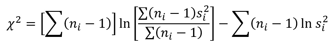
The test statistic for Bartlett's test is B, but it is distributed as χ2 with a - 1 degrees of freedom, where a is the number of samples being compared. Naturally, for a 2-sample t-test, a = 2. Your book employs k as the notation for the number of samples, but I like to change things up to keep you on your toes. The calculation for Bartlett's test is as follows:
Once again, this formula (which you will be using) differs from that in your textbook, equation 10.44 (which you will not be using), and for the same reason as before. The procedure outlined by your textbook calculates the pooled sum of squares first, and that step is included in this formula. Dividing the formula above into 3 parts (which would be a very useful approach to your calculations), the first part, delineated by the first set of squared brackets, is simply the sum of n - 1 for all of the samples. The subscript i is the sample number, where i ranges from 1 to a. The second part of the equation is the natural log (ln) of the pooled sum of squares. The natural log can be found easily in Excel as: =LN(value). From the product of these 2 parts is subtracted the sum (across all samples) of the natural log of the variance times n - 1.
As if the calculations weren't cumbersome enough, if the resulting χ2 value is close to the critical value, then a correction factor C must be applied, where:
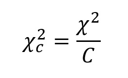
This value can then be compared to the critical value for χ2 at a - 1 degrees of freedom (v). These critical values can be found in Table B.1 in your textbook (page 672 in the 5th edition). The null hypothesis is that the variances are equal. The test is one-tailed, so use the α = 0.05 value, and not the α = 0.975 and α = 0.025 values. If you found that last sentence confusing, you will want to review last week's assignment...
Question 7: Use Bartlett's test to determine whether or not the homogeneity of variance assumption is met for the data for Example 8.1. Remember that you do not have to apply the correction factor unless your Chi-square value is close (within a few tenths) to the critical value. Also remember the advice given previously: break the formula up into separate calculations, and put the resulting values back together to get your final answer.
Having worked through that, you will now greatly appreciate the simplicity of Hartley's Fmax- test. This is the test that we will use to test for homogeneity of variance for the rest of the semester because it is "quick and dirty". It isn't a bad test, and I have been known to use it on occasion, but for publishable data, you really should make use of Bartlett's test, especially if you are using a software package to analyze your data. That said, to use the Fmax-test, simply divide the largest sample variance by the smallest sample variance, and compare the ratio to THIS table, which uses k to denote the number of samples being compared. If you have unequal sample sizes, use the degrees of freedom (n - 1) from the smallest sample in the ratio that you calculated. This also is a one-tailed test, and so values for the variance ratio exceeding the critical value on the table will result in rejecting the null hypothesis that the variances are equal, at α = 0.05.
Question 8: Use Hartley's Fmax-test to determine whether the assumption of homogeneity of variance is met for the data for the shorebird data and the goose data.
If the homogeneity of variance assumption is not met for a 2-sample t-test, but the data are normally distributed, there is a t-test (Welch's approximate t-test) that can be applied. If, however, the data are not normally distributed, and cannot be transformed (we will discuss this another day) to meet the assumption of normality, we will be forced to use a nonparametric test. These typically make use of ranks instead of the raw data, and are less powerful than parametric tests, but they do not require the same assumptions as the parametric tests. The nonparametric equivalent of a 2-sample t-test is the Mann-Whitney test.
The Shapiro-Wilk results for the shorebird data were W = 0.983 (p = 0.930) for the tern data and W = 0.933 (p = 0.223) for the avocet data, so the normality assumption is met for that comparison. The goose data on the other hand (W = 0.317; p < 0.0001 before and W = 0.700; p < 0.0001 after), definitely do not meet the normality assumption, and so we would be better served by applying the Mann-Whitney test (section 8.11, p.163 in the 5th edition).
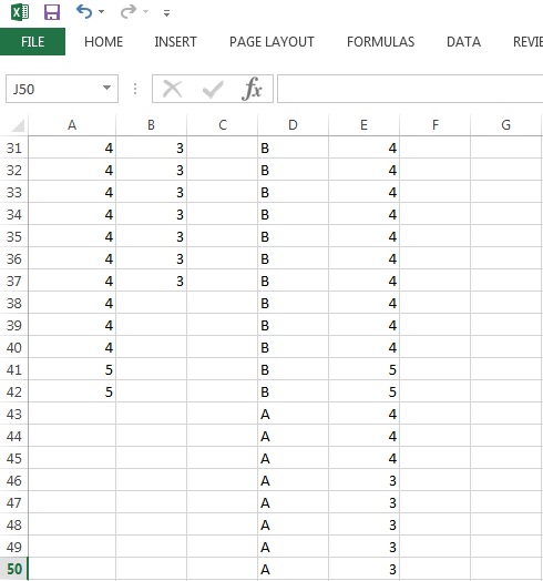
The first step is to get ranks for the data. Counterintuitively (for me at least), the highest values get the lowest ranks, and the lowest values get the highest ranks. Identical values receive tied ranks, where they all receive the mean of their rankings. For example, if a sorted (highest to lowest) array of data has the same value for observations 4-8, they all would be assigned a rank of 6. Excel will create rankings for you, provided that you have first organized the data into a single column. First, copy and paste the data from column A into a new column (e.g., column E). Then, to the left of those data (column D in my example), fill each cell in the column with the letter "B" (for "before"). You should be able to do this by typing it in the first cell, and then dragging it.
To add the "after" data to this, copy the observations from column B, and paste them below the observations for the "before" data. Then fill the adjacent column with the letter "A" (for "after"), and copy that down. Here is an example of what it should look like:
To generate ranks for the data, we can use the RANK.AVG function, which assigns tied ranks the mean rank value. To get ranks for the data, type the following into a cell to the right of, but in the same row as the first observation (cell F3 in my example):
=rank.avg(E3,E$3:E$77)
These cell positions are for my example. If your data have different locations, you will have to adjust the formula accordingly!
The first value is the cell containing the observation that you wish to rank, and the range following the comma defines the reference observations. This range can be selected by highlighting the observations with the mouse, but take note of the anchors present in the formula. These anchors have to be added before the formula is copied so that all observations are ranked relative to the same series of observations. Copying the formula down should reveal that the tied-ranks criterion will produce the same number of ranks as there are levels of the observations.
Now the sum of the ranks can easily be determined for each of the two groups, by, well...summing the ranks for each of the two groups.
For the Mann-Whitney test, we calculate 2 test statistics, U and U', as follows:
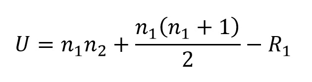
Where n1 and n2 are the sample sizes for the first and second sample, and R1 is the sum of the ranks for the first sample, and:

Where, R2, is the sum of the ranks for the second sample.
Both values (U and U') are compared to the critical values for U (Table B.11, page 747 in the 5th edition), and if either value (you can save time by comparing only the highest value) meets or exceeds the critical value at the appropriate level of α, then the null hypothesis is rejected. Remember to use the next lowest value for degrees of freedom (or in this case, sample size) if your specific value(s) are not represented in the table.
Question 9: Compare the clutch size data for the snow geese using the Mann-Whitney test to determine whether there was a significant decrease in clutch size after the pipeline spill. How do these results compare with those from the 2-sample t-test?
One last, but important topic left to consider is repeated measures analysis...
Send comments, suggestions, and corrections to: Derek Zelmer